Time Series Analysis GitHub

• Tesla Stock Forecasting by Time Series Models By getting the Tesla Company’s stock information (NASDAQ: TSLA) through the Yahoo Finance. This project will apply the time series analysis methods to investigate the TSLA’s basic information, decompose the TLSA’s time series.
• The exponential smoothing methods to forecast the TSLA’s price in the coming 365 days, and then will use
• The ARIMA model to predict the price. This project also will check the Then we forecast error distribution to check the model’s performance.

Decompose the Time Series

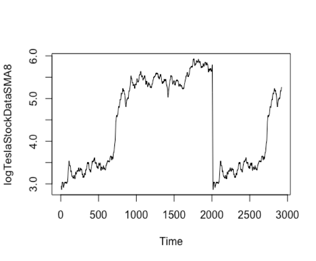
Decomposing a time series means separating it into its constituent components, which are usually a trend component and an irregular component, and if it is a seasonal time series, a seasonal component. For the TSLA stock information, from the price trend plot figure, we can see that there is not seasonal component inside the data. But this time series data should include a trend component and an irregular component. Decomposing the time series involves trying to separate the time series into these components, that is, estimating the trend component and the irregular component. We will SMA() function to smooth TSLA data. We will choose the different order (n=8 and n=40) to check the trend component. The goal is that we try to smoothed the data with a simple move average.

Forecast Model and Evaluation: Exponential Smoothing

• Exponential Smoothing Model Exponential Smoothing model can be used to make the short-term forecasts for time series data. From the TSLA data, we know it can be described as the additive model with no seasonality. From the trend chart, we can see the random fluctuations in the time series seem to be roughly constant in size over time. So we will use the HoltWinter() function to fit a simple exponential smoothing prediction.

7.1.2.2 Evaluation

As a measure of the accuracy of the forecasts, we can calculate the sum of squared errors for the in-sample forecast errors, that is, the forecast errors for the time period covered by our original time series. The sum-of-squared-errors is stored in a named element of the list variable

• logTeslaStockDataForecast$SSE

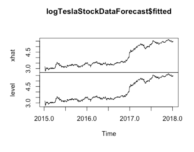
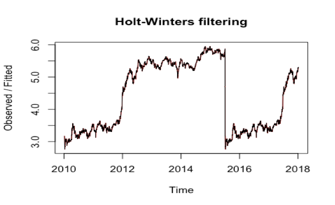The forecast errors are stored in logTeslaStockDataForecast$residuals. HoltWinters(). If the predictive model cannot be improved upon, there should be no correlations between forecast errors for successive predictions. In other words, if there are correlations between forecast errors for successive predictions, it is likely that the simple exponential smoothing forecasts could be improved upon by another forecasting model. 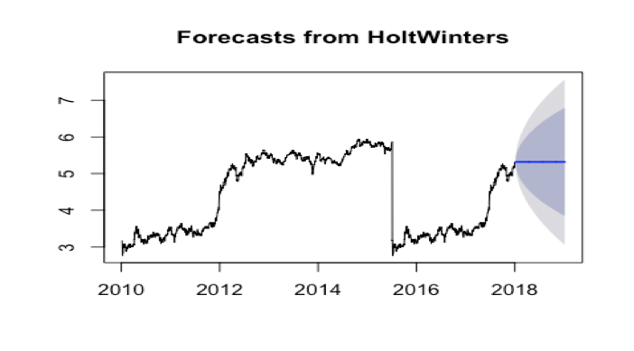To figure out whether this is the case, we can obtain a correlogram of the in-sample forecast errors for lags 1-40 and calculate a correlogram of the forecast errors using the “acf()” function in R. To specify the maximum lag that we want to look at, we use the “lag.max” parameter in acf(). To test whether there is significant evidence for non-zero correlations at lags 1-20, we can carry out a Ljung-Box test by using the “Box.test()”, function. The maximum lag(40) that we want to look at is specified using the “lag” parameter in the Box.test() function. Box.test(logTeslaStockDataForecast2$residuals, lag=40, type=”Ljung-Box”) Here the Ljung-Box test statistic is 31.42, and the p-value is 0.832, so there is little evidence of non-zero autocorrelations in the forecast errors at lags 1-40. To be sure that the predictive model cannot be improved upon, it is also a good idea to check whether the forecast errors are normally distributed with mean zero and constant variance. To check whether the forecast errors have constant variance, we can make a time plot of the in-sample forecast errors: plot.ts(logTeslaStockDataForecast2$residuals) We will use plotForecastErrors() to check whether the forecast errors are normally distributed with mean zero, we can plot a histogram of the forecast errors, with an overlaid normal curve that has mean zero and the same standard deviation as the distribution of forecast errors. The plot shows that the distribution of forecast errors is roughly centered on zero, and is more or less normally distributed. It is plausible that the forecast errors are normally distributed with mean zero. The Ljung-Box test showed that there is little evidence of non-zero autocorrelations in forecast errors, and the distribution of forecast errors seems to be normally distributed with mean zero. This suggests that the simple exponential smoothing method provides an adequate predictive model are probably valid. ![ts_hist(ts_hist.png)]

Forecast Model and Evaluation: ARIMA Model

ARIMA Model

ARIMA (Autoregressive Integrated Moving Average) is a major tool used in time series analysis to attempt to forecast future values of a variable based on its present value. ARIMA(p,d,q) forecasting equation: ARIMA models are, in theory, the most general class of models for forecasting a time series which can be made to be “stationary” by differencing. ARIMA models are defined for stationary time series. Therefore, if you start off with a non-stationary time series, you will first need to ‘difference’ the time series until you obtain a stationary time series. To difference the time series d times to obtain a stationary series, we use the diff() function. Then we will use the A formal ADF test does not reject the null hypothesis of non-stationarity, confirming our visual inspection:

• Stationarized the Time Series adf.test(logTeslaStockData)

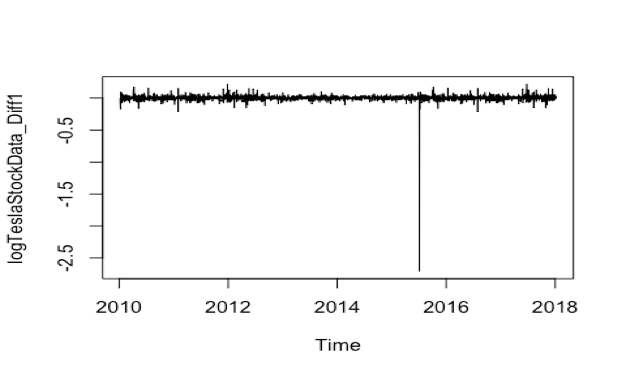
We can see the ADF.test result. Before diff(), the p-value is 0.7165 and after diff(), the p-value is 0.01. So logTeslaStockData_Diff1 is the stationary time series and ready for ARIMA model. The next thing we will plot the ACF and PACF value. acf(logTeslaStockData_Diff1, lag.max = 40)

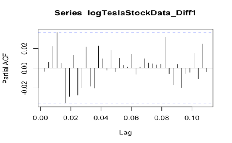
Evaluation

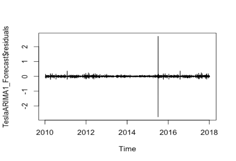
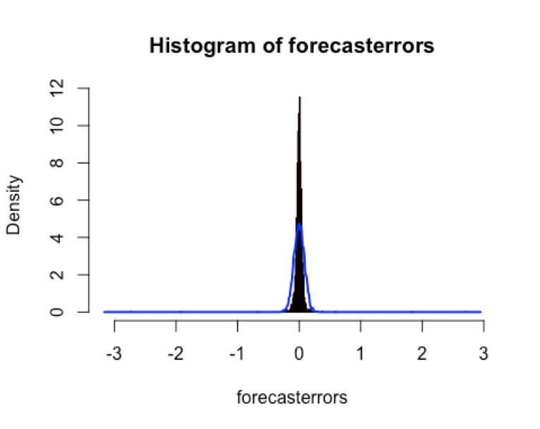
We still use plotForecastErrors() to check whether the forecast errors are normally distributed with mean zero, we can plot a histogram of the forecast errors, with an overlaid normal curve that has mean zero and the same standard deviation as the distribution of forecast errors.

plot(TeslaARIMA_Forecast$residuals) The plot shows that the distribution of forecast errors is roughly centered on zero, and is more or less normally distributed. It is plausible that the forecast errors are normally distributed with mean zero. This suggests that the simple exponential smoothing method provides an adequate predictive model are probably valid.

ARIMA Model discussion

In this case, we use the auto.arima() to forecast the price. But the model parameters show the model is ARIMA(0,0,0). So, we can be sure that there is white noise in this time series data. So it means that the errors are uncoorelated across time, but is does not imply the size of errors or indication of good or bad model. So based on natural log time series data, we will choose ARIMA(0,1,0) to forecast the price. Comparing with the result of ARIMA(0,0,0), ARIMA(0,1,0) has better result. It proved the we should be very careful to choose the auto.arima and choose right parameter to build the forecast model.

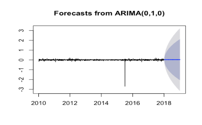
Summary

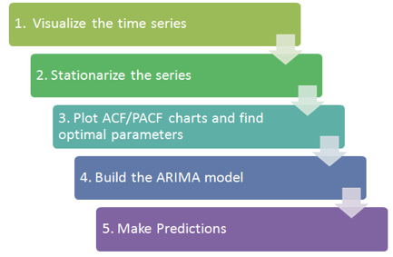
In this section, we use the TESLA stock data as time series. We decompose it and use the HoltWinter exponential smoothing and ARIMA to forecast the future stock price. The basic procedures are as the following figure.

The other thing is we should always to analysis the errors and tune model parameters to achieve the better results.